Throughout much of the 20th century, frequentist statistics dominated the field of statistics and scientific research. Frequentist statistics primarily focus on the analysis of data in terms of probabilities and observed frequencies. Causal inference, on the other hand, involves making inferences about cause-and-effect relationships, which often goes beyond the scope of traditional frequentist statistical methods.
Causal inference has a long history, but it gained more prominent attention in the latter half of the 20th century. This increased interest was partly due to advancements in statistical methods and the development of causal inference frameworks. In the 1980s, the work of Judea Pearl on causal inference significantly contributed to the field which continued into the 21st century. Economists and social scientists were among the first to recognize the advantages of these emerging causal inference techniques and incorporated in their research.
However, based on my personal anecdote, the data science community didn’t truly prioritize causal inference until around 2015 or later. It was during this period that less technically oriented economists faced significant challenges related to the scaling of big data, prompting them to seek assistance from data scientists. Unfortunately, data scientists often lacked the necessary expertise in causal inference, resulting in limited knowledge transfer to business stakeholders. As a result, we, the data scientists, missed an important development for quite a bit, so let’s catch up on that!
What is causal inference?
 New York in the parallel worlds
To explain causal inference, I like an analogy of a parallel or alternative world. Nowadays, with the help of GenerativeAI, we can really simulate or create new worlds. Have you ever wondered how New York would be if the Aztecs would take over of Americas? Or what if the Roman Empire still ruled the world?
Now, how does this relate to data science and business decisions? Well, businesses make important choices every day, like where to invest money, who to hire or fire, and what the consequences of public policies might be. The data they collect only shows one side of reality. To really understand the results of their decisions, they need to explore an unseen or simulated reality. That’s where causal inference comes in, helping us make better decisions by considering alternative outcomes.
Let’s take an example to make it clear. Imagine you’re in charge of expanding the business of a company that makes snack bars for kids. Your goal is to boost sales, and you’re considering adding more sugar to your products because you have a hunch that kids love sugar. After enchancing all your snacks with sugar, you want to measure its impact. You want to know how much your sales would be in a parallel world where kids were stuck with bland snacks compared to your sweet treats. This is where causal inference steps in to provide the solution.
 Sales of sweet snacks vs bland snacks
The chart above illustrates the difference between an observed scenario represented by the red line and an unobserved scenario represented by the black line. The technical term for the black line is ‘counterfactual’—it represents what the sales would be if we didn’t enhance the snacks with sugar.
To continue this intriguing story, let’s fast forward a bit. Now, you’re the CEO of the same company, which has gained international recognition and is traded on stock markets worldwide. However, recently, some pesky Facebook groups formed by moms and dads have launched a public campaign, claiming that your products and the entire concept behind them are making their children overweight and prone to diabetes.
In an effort to address these concerns and launch a PR campaign, you reach out to a university with whom you’ve collaborated in the past to improve your products. You ask them to investigate these claims. To your surprise, they request the same sales data that initially sparked the sugary product campaign. A few nights later, an underpaid PhD student conducts a causal inference analysis, constructs counterfactuals and uncovers the following findings.
 Percentage of people with diabetes, simulated data
Upon seeing these results, you become convinced that there is a conspiracy against you and your company. You quickly instruct your lawyers to halt any further funding to the university and come up with a plan to take legal action against all parties threatening you. From this intriguing tale, we can take two valuable lessons about how Causal Inference played a pivotal role in two critical business scenarios:
- Assesing the impact on sales by adding more sugar to your products.
- Assessing the effects of a sugary diet on children’s health.
Here are more examples of causal inference:
- Effect of attending a data science meetup on a person’s future and earnings
- Air quality and free public transport
- Percentage of electric vehicles and air quality
- Impact of your campaigns (sales, marketing or support) on the revenue, profit, employees satisfaction and etc.
- A product or service price change on the demand
Running a causal inference analysis
 Looking back at our fictional story, the lawyers could raise a valid argument that association or correlation doesn’t necessarily imply causation. In simpler terms, just because there’s a correlation between high sugar consumption and an increase in the number of people with diabetes doesn’t mean that one directly causes the other. It’s another case of a spurious correlation, isn’t it? Take, for example, the high correlation between umbrellas and wet streets. Does that imply that people with umbrellas cause puddles on the streets? Of course not. It’s more likely that a common factor, in this case, a rain (or, using the technical term, a confounder), affects both variables. Now, the question is how can we estimate the impact given that there is a causal link between diabetes and a sugary diet?
One approach to understanding the impact of sugary snack consumption on diabetes risk would involve conducting an experiment. In this experiment, children would be randomly assigned to receive either unsweetened or sugary snacks. After a decade, we’d analyze how many children developed diabetes in each group and calculate any observed differences. If differences exist, we could confidently attribute them to causation since the random assignment eliminates biases. However, I can already see parents rolling their eyes and rightly questioning my moral values. And they’re correct - we can’t conduct cruel experiments on children or people. Secondly, it would take 10 years to figure out the difference, and thirdly, there are other biases to consider. Last but not least, it would be really expensive.
Linear regression
Let’s set aside for the moment the need to estimate causal impact and explore modeling the problem using linear regression. If we represent snack consumption as a binary variable (sugary or not), we can proceed as follows:
Now, here comes the exciting part – we can enhance our model by incorporating all the additional variables available to us. In our example, we might have access to demographic data, an individual’s activity or behavioral information. For instance, we can consider factors like how frequently and for how many hours a person exercises each week, their dietary habits, and so on.
\(X_i\) denotes extra variables what we might include
You might be wondering whether adding more variables to the model is a good idea, and the short answer is: it depends. When dealing with a causal question, it’s crucial to include variables known as confounders. These are variables that can influence both the treatment and the outcome. By including confounding variables, we can better isolate and estimate the true causal effect of the treatment. Failing to add or account for confounding variables may lead to incorrect estimates.
 Example of a confounder
Additionally, including variables that are only predictors of the outcome can be beneficial. It reduces the variance and allows for a more precise estimation of the causal effect. However, adding a variable that predicts only the treatment can lead to a less accurate estimation of causal effect. This occurs because it increases the variance, making it more challenging to estimate the causal effect accurately.
It is worth to emphasize, that a regression model gives an average estimate based on the given inputs. In causal inference, this outcome is referred to as the average treatment effect, \(ATE\), which provides an estimation across the entire group, rather than on an individual basis. Depending on the problem at hand, you might need to estimate an individual treatment effect. The Synthetic Control method, discussed below, allows you to assess the impact at an individual level.
Causal graphical models
Now that we’ve discussed the cases to consider, let’s dive into the process of deciding which variables to include and which to omit in your model. Causal graphical models, championed by Jude Pearl since the 1980s, offer an appealing approach at first glance. The fundamental concept is to construct a Directed Acyclic Graph (DAG) that contains all variables in your analysis. Using this graphical representation you can make informed decisions about which variables to retain and which to exclude.
In this framework, each node in the graph represents a variable, and an arrow pointing to another node signifies a causal relationship. The process of constructing this graph involves utilizing three building blocks: a pipe, a fork, and a collider, which help describe the causal flow between variables. This approach forces you to engage in a thoughtful and clarifying exploration of your model’s causal structure.
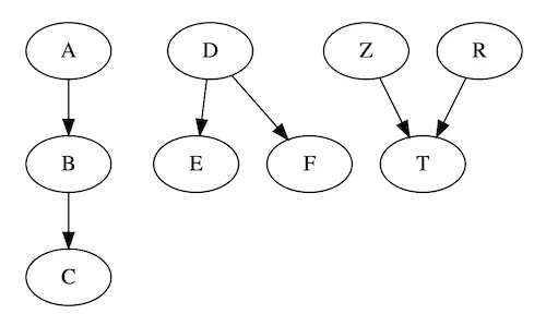 From left to right: a pipe, a fork and a collider
While learning about causal graphs can be challenging, it offers substantial benefits in understanding and addressing various causal inference problems and their solutions. Some argue that this approach doesn’t scale well on a model with +20 input variables. In my experience, most of the time we start with a limited set of variables and build the derivatives of these variables. Therefore, there is an opportunity to build a structural map on the primary variables in most of the cases.
Additionally, to alleviate the pain and speedup process, frameworks such as DoWhy and econml have been developed. In summary, starting your modeling journey with a causal graph may indeed be a challenging task, however it is a proven framework to get a robust and insightful model.
Instrumental Variable
 In a nutshell, the causal graph should facilitate a solution of a causal problem. However, there many methods to tackle the problem depending what data and challenge you have at hands. Instrumental Variable (IV) method is quite unique. In theory, it seems like a magical solution — you find a variable that has a causal link to a treatment, but doesn’t impact the outcome directly, and voilà, you’ve cracked the code of causation. However, there’s a crucial requirement: the IV must remain completely unrelated to any unobservable factors. This means you need prior knowledge ensuring that the treatment and the outcome have no connections with any variables — an undertaking that can be quite challenging, if not nearly impossible, in the real world. In my experience, I haven’t come across any instances of its use, but interestingly, nearly every causal inference course dedicates a chapter to this intriguing concept.
Difference in Differences
DiD is a straightforward method that can be implemented in Excel without the need for advanced tools. The concept revolves around comparing two versions of a subject or a unit under investigation: one before a particular event or treatment and the other after. To enhance the analysis, you introduce a control group — a similar entity that remains unaffected by the treatment.
 What are the potential effects of a young girl taking her chemistry classes seriously
Let’s consider an illustrative example: before the introduction of the free transport policy in San Diego, the average air pollution level was 10. After the policy was implemented, it decreased to 8. However, we can’t simply subtract 10 from 8, as it would yield biased results. To address this issue, we turn to data from a neighboring city, Tijuana, located just across the border. In Tijuana, the pollution level before the policy was 11, and after its introduction, it dropped to 10. Notably, Tijuana was not affected by the policy. Applying this approach, we find that the bias reduction diminishes the impact from \(-2\) to \(-1\).
\[diff = (SanDiego_{after} - SanDiego_{before}) - (Tijuana_{after} - Tijuana_{before}) =\] \[(8 - 10) - (10 - 11) = -1\]Synthetic control
In our previous example, we made an assumption that the cities were similar, with the treatment being the only differing factor. Furthermore, we simplified the problem by considering only four parameters, which inevitably introduced a degree of uncertainty into our estimation. But what if we had access to a wealth of data from various units (cities in the previous example) and the ability to observe changes over time?

Enter the word of Synthetic Control. Like a magician, we build a synthetic twin for our treatment group. To do that, we take the treatment group and regress against a bunch of similar units, and with regularization, we select the most relevant features and determine their weights.
For instance, let’s evaluate the impact of Mark Zuckerberg having children on teenagers’ happiness in social networks. In order to construct a synthetic control group, we certainly include Bezos, Musk, and Gates, but we might also add Jon from the UK and Guiseppe from France. Never heard of the latter two? That’s precisely the point! With this model, built from data preceding the event (Zuckerberg having children), we project the data into the future, thereby generating our imaginery future, namely counterfactuals, which gives us a way to measure the impact.
 Fictitious example
Previously, we discussed the average treatment effect, a measure that helps us estimate the overall causal impact on a treatment group. Now, with the synthetic control method, it becomes possible to estimate an individual treatment effect (in this case, the effect of Zuckerberg having children), provided that we have a sufficient amount of data to create a synthetic control.
Now, lets magic fade and look at disadvangates of synthetic control. The method assumes that all potential confounding variables are measured and controlled for as with linear regression. The synthetic control method assumes that the pre-treatment data accurately represent the underlying data-generating process. And on top of that, you get the standard ML problems - overfitting, difficult to validate (but not impossible) just to name few.
Double ML
Since the ’90s, when causal inference gained popularity, the data landscape has changed significantly. More often than not, we now find ourselves dealing with enormous amounts of data for a given problem, often without a clear understanding of how all the variables interconnect. In theory, DoubleML can be helpful in such cases.

The DoubleML method is founded on machine learning modeling and consists of two key steps. First, we build a model \(m(X)\) that predicts the treatment variable \(T\) based on the input variables \(X\). Then, we create a separate model \(g(X)\) that predicts the outcome variable \(Y\) using the same set of input variables \(X\). Subsequently, we calculate the residuals from the former model and regress them against the residuals from the latter model. An important feature of this method is its flexibility in accommodating non-linear models, which allows us to capture non-linear relationships — a distinctive advantage of this approach.
\[\tilde{T}_{sugar} = T_{sugar} - m(X)\] \[\tilde{Y}_{outcome} = Y_{outcome} - g(X)\] \[\tilde{Y}_{outcome} = \alpha_0 + \beta_t *\tilde{T}_{sugar}\]Consider using DoubleML when you have high-dimensional data (many features) or when the relationships between inputs and treatment/outcome are not linear. DoubleML is particularly useful when you need to estimate treatment effects that vary across different subgroups or individuals. However, it’s essential to remember that DoubleML cannot magically eliminate the influence of poorly considered confounding variables.
Useful resources
The purpose of this blog post was to introduce readers to the world of Causal Inference and inspire them to explore it further. I’m planning to follow up with a hands-on post using public data. Below, you can find a list of resources that I found helpful during my own journey of learning about Causal Inference.”
-
Causal Inference for The Brave and True. It’s freely available on the internet, hands-on focused, and presents easily understandable formulas.
-
Mastering mostly harmless econometrics. A very nice introduction to Causal Inference. (video)
-
 Causal Inference in Python: Applying Causal Inference in the Tech Industry
 -
 The Book of Why by Judea Pearl, the inventor of causal diagrams, not only delves deep into the theory but also offers valuable insights from a historical perspective.