A causal analysis ran on the traffic data collected in Luxembourg, a small and green country in Western Europe, indicates that a 1% increase in traffic leads to a 0.45% rise in nitrogen dioxide (NO2), a major air pollutant primarily emitted from cars and factories. Elevated levels of NO2 can adversely affect health in various ways. It can make breathing problems worse, negatively impact heart health, increase susceptibility to infections, and particularly affect vulnerable groups such as individuals with asthma, children, the elderly, and those with existing heart and lung conditions.
In the air quality directive the EU has set two limit values for NO2 for the protection of human health: the NO2 hourly mean value may not exceed 200 micrograms per cubic metre (µg/m3) more than 18 times in a year and the NO2 annual mean value may not exceed 40 micrograms per cubic metre (µg/m3).
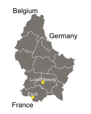
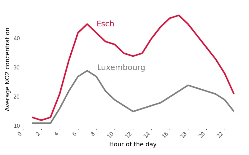
The data for this analysis were collected from two different locations in Luxembourg, each about 30 kilometers apart. In both locations, traffic and air quality sensors were placed in close proximity to provide accurate measurements of traffic-related pollution. Among these, the city of Esch sur Alzette stands out. Despite having similar traffic counts as the other location, Esch sur Alzette consistently shows higher pollution levels. This difference could be attributed to the city’s history of being surrounded by heavy industry. Interestingly, at night, pollution levels between the two locations tend to converge, indicating that the elevated pollution in Esch sur Alzette fluctuates with daily activities and is not a constant feature.
Recommendations

The results of the causal analysis can be used to precisely control traffic overflow in hotspot areas. They can help calculate a range of traffic values, and upon nearing maximum capacity, traffic can be diverted through alternative routes. In the case of exceeding the maximum allowed CO2 levels, we can calculate how many vehicles need to be diverted from the affected area to normalize the pollution levels.
The quesiton is if it feasible as Luxembourg has already invested in traffic flow optimization - it offers free public transport nationwide, and numerous upgrades have been made to roads and other transportation links. Yet, these improvements do not alleviate the high pollution levels in areas at the crossroads with France. Any enhancements, such as increased highway capacity or better traffic management, are quickly offset by an influx of more vehicles.
For residents in highly polluted areas, the advice might be to relocate. However, these areas are known for their lower real estate prices, making relocation impractical for many.
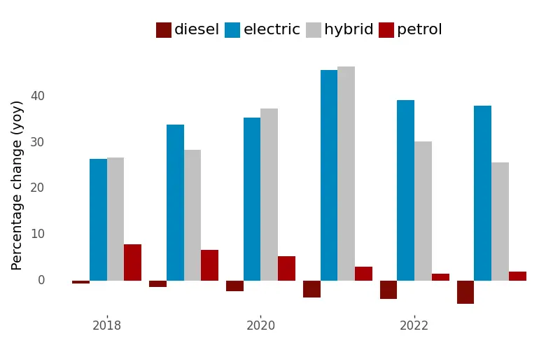
Additionally, a nation goal should be to decrease the number of older-generation cars and ideally replace them with electric vehicles (EVs). The chart below shows that the percentage growth of EVs in Luxembourg is impressive - around 35% for the last 4 years. At the same time, the prevalence of diesel and petrol cars is declining. However, their absolute numbers remain high, with 268000 diesel and 237000 petrol cars. Assuming a consistent growth rate, it will take about 8 years for EVs to reach the current levels of diesel and petrol cars, starting from the current count of 23400 EVs. On a positive note, not all older cars are in active use, despite being registered. Additionally, while newer-generation cars emit fewer pollutants than their older counterparts, they are not entirely NO2 neutral.
Data
As mentioned earlier, the data was collected from two different locations where the NO2 sensors and traffic counters were situated approximately 700m-800m apart. Both locations are in proximity to a city. The traffic and pollution data were acquired from data.public.lu - a public data repository of the Luxembourg government. The weather data was obtained from a third party, as data.public.lu does not currently provide it, but plans to do so in the second half of 2024. For the analysis, the following filters were applied:
- The date range is from 2020-03-01 to 2022-12-31, as earlier data is very sparse and, presumably, unreliable.
- The models are built on rush hour data, spanning from 7:00 to 21:00. Early investigations indicated that the data distributions for night and day are quite different; therefore, they were modeled separately.
A simple regression model
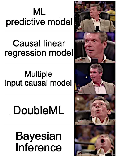
In this analysis, I explored various methodologies, all tied to a causal question: what is effect on NO2 pollution with a one percent rise in traffic. The need for causal inference comes from the limitations of simple linear regression, which often yields inaccurate or biased results, preventing reliable conclusions from mere traffic and NO2 data correlations. An alternative approach, a controlled experiment involving random assignments of vehicle passage near sensors, while methodologically sound, is impractical to implement.
Let’s begin by considering a simple linear regression model, where we assume that NO2 pollution is solely driven by traffic.
\[log(pollution) = \alpha + \beta * log(traffic) + \varepsilon\]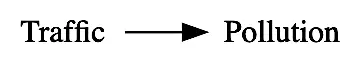
The estimate of \(beta\) or the slope of this model, gives us 0.4898 or 0.48% effect and \(R^2\) is 0.1851 meaning that only 18.5% variability can be explained with this simple model. But let me remind you, that this approach captures the total effect on NO2 and potetially it means that we overlook other potential confounding factors. For those unfamiliar with the term, a confounder is a variable that influences both the outcome (in this instance, pollution) and the independent variable of interest (in our case, traffic).
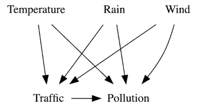
From extensive research on NO2 pollution, we know that major contributors include cars and factories. In my analysis, I have considered the following variables as potential confounders:
- Air temperature: Temperatures below 0°C may lead individuals to turn on heating, some of which might still use coal or other ‘dirty’ materials. This also affects traffic - we can expect more cars during both cold and hot days.
- Wind speed: High wind can lower NO2 concentration in an area. However, the absence of wind, combined with a sunny summer day, might increase NO2 concentration. Windy days, perceived as unpleasant, might also increase traffic.
- Precipitation: Rainy days might affect both NO2 concentration and traffic flow.
- City code: Due to varying landscapes and urban planning, different cities are expected to have distinct effects on traffic and pollution. For example, Luxembourg City has many valleys where pollutants can be trapped.
- Time (omitted from the analysis): Initially, including time variables such as hour, workday, month, and year might seem beneficial due to the high seasonality in the dataset. However, the traffic data captures the seasonality very well and time doesn’t have a direct effect on the pollution levels.
An advanced regression model
The additional features outlined above allow us to build a causal graph and more precisely estimate the effect of the treatment group, namely the traffic. The estimated effect is 0.4505 or 0.45%, which is 0.03% lower than that estimated by the simple model. Meanwhile, \(R^2\) has increased to 0.48, which is a positive development.
Beyond yielding more accurate estimates, the multiple input model offers detailed insights into each variable. Consider the table presented below:
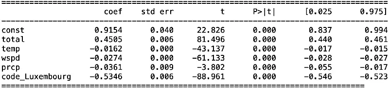
Of particular interest is the code_Luxembourg variable. This indicates that, on average, the difference in pollution levels between Esch sur Alzette city and Luxembourg is 54%. Essentially, this implies that the model estimates a 54% reduction in pollution levels in Luxembourg compared to Esch sur Alzette, assuming all other variables remain constant. Furthermore, the model shows that an increase in precipitation, wind speed, or temperature leads to a decrease in NO2 pollution by 3.6%, 2.7%, and 1.6%, respectively.
A double ML model
 I have incorporated a DoubleML model into the analysis, recognizing that it may not be a perfect fit for the problem at hand. A key selling point of this approach is its ability to handle high-dimensional data and effectively manage a large number of potential confounders. Supposedly, DoubleML reduces the necessity for deep domain expertise, allowing one to construct models even with a basic understanding of the system and data, provided there is ample data and some familiarity with machine learning techniques. My contention, however, is that constructing a theoretical model is still feasible and beneficial. For instance, in this analysis, we can derive numerous variables from the ‘datetime’ variable, such as year, month, and day of the week. Yet, in constructing a theoretical model, we could simply use a consolidated time variable to gauge its overall impact on the system.
While the DoubleML approach might be excessive for the current problem, its practical implementation reveals several issues. First, the model primarily yields estimates on the interaction between the treatment and the outcome, but it does not inherently provide insights into other parameters like city, temperature, or rainfall. This means additional steps are needed to analyze these factors. Second, the complexity of the DoubleML implementation can obscure the model’s internal workings, leading to a reliance on superficial understanding. Users must trust the model’s outcome without fully grasping the underlying mechanics.
The implementation of a DoubleML model is relatively straightforward. First, you build a model to predict the treatment using the input variables. To capture non-linear relationships, any modeling technique can be employed. In my analysis, I utilized XGBoost. We build the model on a training dataset and then make predictions on the test set. However, our focus is on the residuals, i.e., the difference between the true values of the test set and the predicted values.
Next, we proceed to calculate the residuals of the outcome model, constructed without including the treatment variable.
Finally, we obtain our estimate via a simple linear regression:
The result is 0.44 which is close to the estimate of the multiple input regression model at 0.45, however \(R^2\) is lower at 22.5%
Bayesian inference model
 To me, Bayesian inference is an ideal complement to Causal Inference. Firstly, there’s a nuanced difference in how Bayesian inference presents estimated parameters compared to frequentist frameworks. Frequentist confidence intervals indicate the range within which we would expect the true parameter value to fall in repeated samples, not the probability of the parameter being within that range in a given sample. In contrast, Bayesian credible intervals offer a probability-based interpretation: they indicate the likelihood of the parameter being within a certain range, given the observed data and prior knowledge.
Secondly, we can incorporate existing knowledge about the system under study. In our case, we know the following:
- The NO2 pollution rate is always positive.
- A positive relationship exists between traffic count and NO2 pollution.
- Traffic count can’t be negative.
- The log-normal distribution can be used to describe the NO2 pollution rate.
The Bayesian model definition almost identical to the multiple input regression model described earlier, except that we need to encode priors which we defined above.
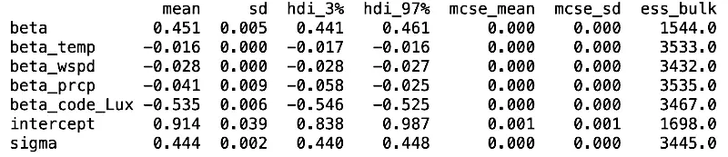
\[log(pollution) \sim Normal(\alpha + \beta_t * traffic + \beta_c * city + \beta_{temp} * temp + \beta_w * wind + \beta_p * prcp)\] \[\alpha \sim HalfNormal(5)\] \[\beta_t \sim LogNormal(0, 3)\] \[\beta_c \sim Normal(0, 2)\] \[\beta_{temp} \sim Normal(0, 2)\] \[\beta_w \sim Normal(0, 2)\] \[\beta_p \sim Normal(0, 2)\] \[\varepsilon \sim HalfNormal(1)\]The table below presents the results from the Bayesian inference. The estimated parameters align closely with those obtained from previously described methods. A significant enhancement, however, is the inclusion of credible intervals for each parameter. Specifically, the estimated effect of traffic on NO2 is 0.451, with a credible interval ranging from a lower bound of 0.441 to an upper bound of 0.461. This approach, with its emphasis on credible intervals, represents the correct and most informative way to report such results.
Useful resources
- For those interested in replicating the analysis, which is highly engouraged, or simply exploring the model implementations, I have shared my notebook on GitHub.
- A highly recommended resource for understanding Causal and Bayesian Inference is the following book, which I found extremely valuable:

Final remarks!