
In the last decade or so, the online retail business has become completely liberated - anyone with a product idea can start selling with minimal investment. Typically, the process unfolds as follows: source an idea, which might be an improvement on an existing product or a copycat of a bestselling item from other marketplaces such as Temu or Alibaba, then purchase or manufacture in China and ship it to a local warehouse. With the rise of smart manufacturing, local production of some products has become more cost-effective, and there are instances where sellers prefer labels that reference local origins. However, despite these developments, China continues to be a dominant global manufacturing hub.
With the product in hand, a seller embarks on the challenging journey of product promotion. To accelerate sales, a seller allocates a budget for promoting the product directly on a marketplace or uses Google and/or social platforms to drive customers to their page and make sales. This creates a major objective: reducing the cost of acquiring a new customer while maintaining or increasing sales volume. When speaking to sellers, this strategy is often reiterated like a mantra. However, other options exist, which could lead to higher profit margins, though they may not be immediately apparent to sellers.
Test everything
Experimentation has always been integral to the marketing and sales process. However, in the pre-ecommerce era, changes in packaging, branding, or products took much longer compared to the present, where everything happens in the blink of an eye. Despite this speed, sellers, particularly those with a few successful products, often show resistance to change, whether in pricing or the context of a product. The reasoning is straightforward: if it sells, don’t fix it. Nevertheless, A/B testing, as simple as changing a product background color or text font, offers the opportunity to experiment on a small scale, thereby minimizing the risk of disrupting overall sales while potentially enhancing them. Such tests can be conducted with 1-10% of customers, and if a change results in lower conversion or margin, the situation can be swiftly reverted. Implementing A/B testing is not overly complex. For example, you can create a page nearly identical to the main product page, alter a few details, and direct every tenth customer there. The critical aspect is to gather sufficient evidence that the change leads to a positive impact, e.g. a better conversion rate or higher sales.
 For those looking to elevate their experimentation efforts, the Multi-Arm Bandit method is worth considering. Unlike A/B testing, where routing allocations are fixed until enough data is collected to make a decision, the Multi-Arm Bandit method dynamically allocates traffic based on the most recent performance. It occasionally makes random selections to continue exploring the ever-changing environment. Furthermore, it offers a more efficient approach for exploring multiple options beyond just A and B. Implementing this method may require assistance, but it is particularly valuable in dynamic environments where opportunity cost is a crucial factor.
Price discovery
The methods outlined earlier are important for experimentation, but they don’t specify the optimal price for conducting such experiments. In most of the cases, we want to optimise our sales strategy for one of three criterias - profit, revenue or market share.
In scenarios where you have historical sales data across at least two different price points, you are well-positioned to estimate demand elasticities. This concept, developed in the late 19th century, is based on a straightforward principle: when the price rises, the volume of sales falls for almost any good, but it falls more for some than for others. Conversely, reducing prices often leads to an increase in sales volumes. Thus, by observing how changes in price affect sales volumes, you can begin to understand the price elasticity of demand for your product.
The chart below illustrates how we can estimate price elasticity using five data points of price and sales volume. A simple formula allows us to estimate demand at different price points.
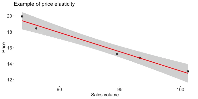
From the example above, let’s take a price decrease from 18.43 to 15.20 where quantities were respectfully 88 and 95. Now we can estimate elasticities:
\[Demand = \frac{(Quantities_{1} - Quantities_{2}) / Quantities_{1}}{(Price_{1} - Price_{2})/Price_{1}} = \frac{(88 - 95)/88}{(18.43 - 15.20)/18.43} = -0.45\]The demand elasticity number is always negative as it reflects the inverse relationship between price and quantity demanded—when the price of a product increases, the quantity demanded typically decreases, and vice versa. In our scenario, the product demand is inelastic—lowering the price by 1% would increase sales by only 0.45%, while raising the price by 1% would decrease sales by the same amount. Therefore, the optimal choice is to maintain higher price levels.
In general, inelastic demand, where the price elasticity is above -1, indicates that customers won’t significantly change their demand if prices increase. For example, necessities like food, water, and electricity are required regardless of price. Similarly, products with addictive components, such as tobacco and alcohol, tend to have inelastic demand. Another case is brand loyalty, with Apple being a perfect example—their products exhibit highly inelastic demand, allowing prices to increase without losing their customer base.
On the contrary, if a price elasticity is -2 or lower, a different approach is needed. In this case, lowering the price will lead to more sales; however, there is a risk that the customer base might quickly shift to a competitor if their price is lower.
So far, we have only considered two price points for a single product, allowing you to estimate demand elasticities with nothing more than a napkin. When dealing with a dozen products and multiple data points, Excel or Python/R/data science tools will prove invaluable. However, scaling up to a larger product portfolio will require a development of a custom model, which offers additional advantages. Firstly, it allows us to factor in the seasonal fluctuations of a product, such as a sales spike in December or slow summer months. Moreover, it enables us to estimate demand elasticities at a higher level, for instance, by product category. The benefit here is that we can apply the elasticities derived from a category to new products within that category. For example, if you have a new herbal tea product, the elasticities of the tea category can be utilized for this new offering.
Examples of application of price elasticities
- Promotions: Businesses often launch promotions to increase market share, enhance product recognition, or boost sales volume. A key question in such scenarios is: How substantial should the discount be? What is the expected sales volume at the new price point?
- Inventory Clearance: Similarly, a campaign may be initiated to accelerate sales for the purpose of freeing up storage space. In this context, determining the optimal price is crucial. What price should be set to achieve the desired results quickly and efficiently?
- Stock Depletion: There may be instances where stock levels drop quickly, posing the risk of running out of inventory. In such situations, increasing prices can help decelerate the sales volume, allowing for time to restock. The important question, however, is by how much to raise the price to decelerate sales without completely eliminating customer demand.
Optimal prices for a portfolio of products
Price elasticities allow us to simulate demand for each product at various price points, enabling the development of a pricing strategy that optimizes for profit, revenue, or both across our entire product portfolio. This approach can also be applied to optimize other key metrics, such as market share or any other objective.
| Price | Sales | Revenue | Profit |
|---|---|---|---|
| 14 | 106 | 1479 | 140 |
| 15 | 101 | 1511 | 144 |
| 16 | 96 | 1533 | 150 |
| 17 | 91 | 1545 | 145 |
| 18 | 87 | 1566 | 130 |
| 19 | 79 | 1501 | 125 |
| 20 | 77 | 1543 | 120 |
The fictitious example above illustrates profit and revenue levels at various price points for a single product. By applying this approach across all products, we can construct the following graph:
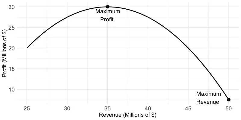
In this example, the maximum profit is $30M. If maximizing profit is our sole objective, we can work backwards to extract the optimal price for each product and implement this pricing strategy. However, if increasing revenue is also a priority, you can move along the curve to the right, allowing for higher revenue with only a minimal sacrifice in profit. For example, at $40M in revenue, your profit will be $2.5M lower than at the $35M revenue point, where profit peaks at $30M. In this case, you would be gaining additional $5M in revenue.
Challenges of applying price optimization techniques
When building a portfolio with optimized prices, we often assume that we can set the price independently of the market. However, this is not always the case. One challenge is competition. If you’re selling an identical or very similar product as a competitor, customers will likely prioritize the lowest price if all else is equal (such as quality, delivery speed, and brand reputation). In such a scenario, lowering your price might help you outcompete the rival if the product has high elasticity (elasticity less than -1). However, raising the price can give your competitor an advantage, allowing them to capture more sales. Similarly, for inelastic products, it can be difficult to increase prices in a competitive market without losing customers to competitors.
So far, we’ve assumed a linear relationship between price and demand. While a log-log model can better capture this relationship, experience shows that deep discounts (e.g., more than 20% off) can attract a significant increase in customers, deviating from the expected demand curve. As a result, price elasticity estimates are more reliable near current price points, but uncertainty increases as prices move further away from these points. This doesn’t entirely invalidate the use of price elasticities, but it is an important consideration to keep in mind.
Finally, if you have limited data points or only a few products, relying on price elasticities and optimization might be premature. In such cases, consensus decisions, such as experimenting with different prices, can provide the data needed to apply the techniques discussed above effectively.
What’s next?
In this blog post, I intentionally focused less on the modeling and implementation aspects to introduce the topic more broadly. If you find price optimization intriguing and want to explore it further, I highly recommend the following book:
 Pricing and Revenue Optimization by Robert L. Phillips